
PEP Macro Approach to Portfolio Construction & Engineering
DEVELOPMENT OF PORTFOLIO CONSTRUCTION CONSTRAINTS
The purpose of this paper is to describe our approach to portfolio construction. While at one level, portfolio construction thinking in the industry is somewhat developed in the form of risk management against a single benchmark mandate, in reality we believe this thinking needs significant revision.
We explain this from first principles in relation to client aspirational objectives. From there, we identify that aspirational objectives imply a particular form. This in turn has a series of implications that creates a depth to mandate constraints that is often absent in portfolio construction.
We also illustrate the importance of mandate constraints in the effective capture of investment manager intellectual property, as a means of translation of the latter into performance that is consistent with the client objectives.
Why so much concern about Portfolio Construction?
An analogy is useful here. Imagine the difference between a large family car and a Formula One car. Both need fuel and both need the engineering for the car itself. The fuel used by the cars is essentially the same, albeit with some performance enhancements for the Formula one car. According to David Tsurusaki, ExxonMobil’s global motorsport technology manager, the difference between the two fuels is like the difference between an off-the-peg suit and having one made bespoke.
The car engineering, however, is a different matter. Each of the cars is engineered to solve multiple objectives. In the case of the Formula One car, these include speed and safety. In the case of the family road car, it’s speed, reliability, safety, comfort and space. These differing objectives and preferences lead to substantially different engineering. Even though the fuel is essentially the same.
Applying this analogy to investment management, the fuel are the investment ideas. How they are used to build a portfolio that “does something”, well that’s engineering. Therefore, portfolio construction does the heavy lifting of engineering the translation of fuel into a portfolio that achieves certain client objectives. One of the challenges in the asset management industry is portfolio construction is historically focused on addressing only one objective. We address this next.
Asset manager mandates and client objectives
Most asset manager mandates take the form of a single market index benchmark, position size constraints and a tracking error (TE) target relative to the benchmark. The emergence of these is perhaps understandable – it provides a degree of clarity to the relationship that is certainly in the interests of the asset manager. It also addresses the practical constraint that, in the absence of a clear benchmark, the client can often criticize the manager for not beating something that in practice had no relevance the mandate – for example, in the event that the market is down, “why did you lose money at all?”. The above simple mandate structure addresses much of these practical relationship problems.
However, it does raise the question of whether the above structure gives the client what they actually want. While at one level, one could argue that what a client wants may be unreasonable, it is instructive to pursue the line of thinking to establish how far a mandate might move in a client’s direction.
Does a client actually want outperformance of a market index? The answer to this is more complicated than may appear. Clients want strong returns – the higher the better. Generally if the market index is down, in itself they have no desire to lose money with the index, albeit that might be the consequence. However, even if a client says they want 8% returns (consistent with long run returns on equities) if the market – or the competition – is up 20%, they will unlikely be happy with 8%. Humans are inherently competitive, and market index benchmarks go some way to addressing this problem. So, from a return perspective, a single benchmark mandate solves a client’s desire for return up to a point – but with a difference in utility for different parts of the return distribution. The utility to low returns on the market index is far lower than at the higher end.
However, there is another dimension to the mandate structure, and that is control. The formal mandate structure allows clients to effect a degree of control over potential negative outcomes, because it constrains the degree to which the manager making a wrong decision could negatively affect the outcome. It also goes some way to make clear whether the manager was right or wrong. This is not a trivial point – investment managers have a tendency to attempt to explain away weak performance as being “early” or because of “temporary adverse market conditions”. The less clear a mandate is, the easier it is for a manager to explain away performance in these vague terms. This is a fundamental mismatch in attitude in the client/investment manager relationship – it is in the client’s interest to maximize clarity, but often the manager has the opposite interest.
Defining client objectives in general terms
So let us attempt to put some structure around client objectives. We believe that most client objectives have the following form, even though they are not reflected explicitly in the mandate itself. They are:
1. Return – for example, produce a return of 10% per annum or more over rolling three- or five-year periods. Or, outperform the long-term benchmark index by 2%-3% per annum over the same horizon.
2. Upside – capture the upside in market returns (benchmark returns) when it is available.
3. Downside – avoid the losses in market/benchmark returns when these occur.
4. Recovery time – minimize recovery time.
Recovery time plays to the idea that clients would prefer to sit in a period of underperformance for as little time as possible. Therefore, it is better (arguably) to lose 10% in a short period of time and recover it all in months, than it is to lose 2% per annum over five years. While the volatility on the second strategy is lower, in practice it is painful for a client to sit with underperformance for five years.
Broadly speaking, most clients would be extremely happy with an investment strategy that addressed all the above objectives. Some might argue this is impractical or unrealistic. However, we do not – developing the idea further illustrates some important points about mandate structure.
Further developing the idea – primary and secondary benchmarks
It should be relatively obvious that solving the upside and downside objectives effectively will automatically solve the return and recovery time objectives (albeit there is a technical point around skew that is significant for recovery time – we address this in the Appendix). Nonetheless, we illustrate this in the table below for a 65/35 S&P/Bloomberg Aggregate benchmark.
The simulated strategy is unrealistic – it is simply designed to show the return improvement for successfully capturing upside and avoiding 50% of downside on both return and recovery time. Therefore, the critical question is how to construct a mandate that addresses this upside/downside challenge.
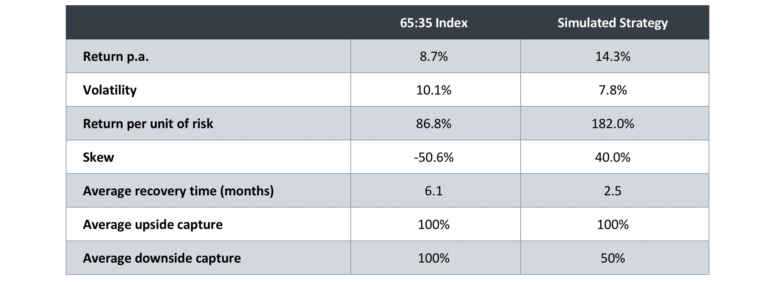
Source: Figures simulated by Public Equity Partners based on data from 01/01/1990 to 09/30/2023. Static benchmark is 65% S&P500, 35% Bloomberg US Aggregate Index in USD. Simulated performance is no indication of future results.
It is fairly easy to see that, relative to the benchmark, the tracking error objectives in each of these two cases (capturing upside and downside) should be different. Subject to knowing that upside is likely to come in the benchmark, the client should focus on capture rather than outperformance, and reduce the TE to minimize the potential for the manager to underperform through active decision-making. Conversely, in the situation where downside coming is a known, the client will wish to maximize flexibility in order that the manager can be as different from the benchmark as possible.
Clearly a single tracking error constraint solves neither of these problems. This therefore describes the inherent problem of making mandates more client-oriented and is the problem we need to solve if the thinking is to progress. The next step requires us to consider something more philosophical.
Do benchmarks express views?
Often benchmarks are considered to be reflective of “no view”, not least because if the manager has no view the logical move is to invest in the benchmark itself. But the reality is a little more subtle than this.
However, investing in a mandate with an equity benchmark does express a view from the client’s perspective. The client believes that equities will produce an appropriate risk-adjusted return, as part of a portfolio, or they wouldn’t be investing in the first place. This view is likely a multi-year view, and importantly has a time horizon longer than the investing horizon of the manager.
To take this idea further, we have seen the emergence of style benchmarks in recent decades. These arguably started with value and growth within equities, but have since extended into a far broader range of styles and asset classes. But these indices capture the same principle as above. They pull out something that is fundamental to the strategy employed by a manager, and therefore operate on a time horizon (arguably infinite) longer than the day-to-day decision making of the manager in terms of security selection.
For example, a value manager may be evaluated against a value benchmark. This is helpful to the client as it helps them understand whether underperformance comes from the style adopted by the manager – which is a longer time horizon view – or the specific decisions made, which operate on a shorter horizon. While the primary benchmark of the mandate for this manager is likely still the broad equity market, the value index is used as a secondary benchmark to help explain performance on the way to outperformance of the primary benchmark.
Drawing these threads together, a secondary benchmark can have the role of expressing a view, on a time horizon longer than the day-to-day manager decisions, about how most effectively to achieve the mandate objectives.
Design of secondary benchmark
There are a number of ways that the secondary benchmark could be designed to reflect the above objectives. But the critical point is it involves expressing a view about when upside and downside tends to happen. Our view is the case that this is influenced by macro factors is very strong. The table below illustrates this for the S&P500.
We have developed a process that produces a prospective view about whether macro forces are expansionary or contractionary, and therefore this view – which operates at a longer time horizon than our day-to-day decision making – can be built into a benchmark.
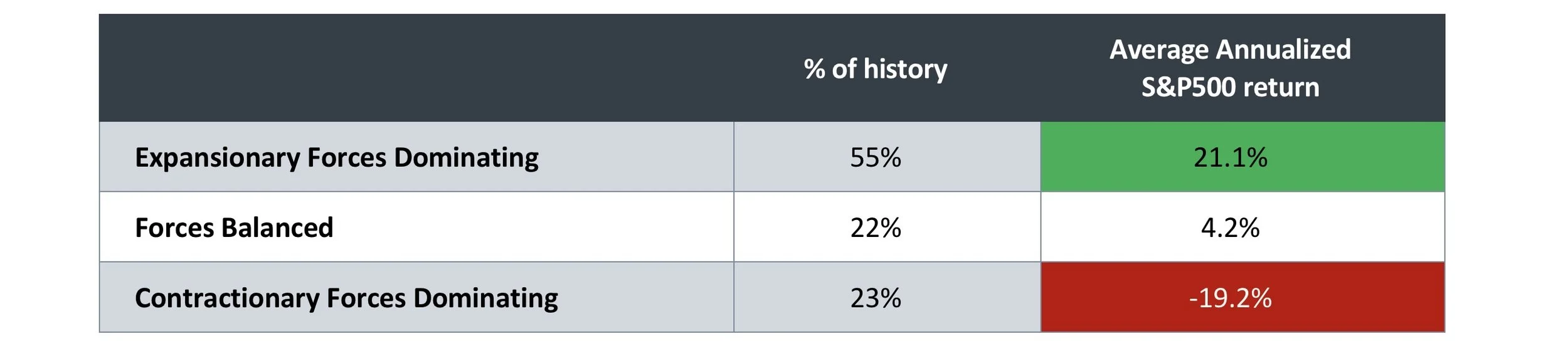
Source: PEP, Bloomberg. S&P 500 in USD from 06/30/1999 to 09/30/2023. Table based on output from PEP’ proprietary models. Past and simulated performance is no indication of future results.
In practice this means that the equity versus bond allocation should change dynamically in the secondary benchmark based on the economic environment.
This ability to change the benchmark structure based on economic environment opens up some additional structural elements that are important to consider. One of these that should be obvious is the benefit on tracking error control:
Tracking error can overall be lower/more controlled relative to the secondary benchmark, than it would be versus the primary benchmark. This is helpful in creating confidence in the control structure.
The tracking error can be lower in upside environments, and wider in downside environments, driven by the economic condition.
Critically, this approach requires clients to “believe” in the philosophy underlying the secondary benchmark design, as it drives the development of everything else.
Additional structural elements
There are some additional factors to consider in the design of the overall structure, which may not be obvious initially, in addition to the asymmetry described above for tracking error:
Symmetry of decision making. Position size constraints should be able to over- and under-weight broadly equivalently relative to the secondary benchmark. For example, if the secondary benchmark can go to 100% in equities, this will often allow underweight but not overweight. This asymmetry is a problem in active management.
Defending to the primary benchmark. The tracking error constraints relative to the secondary benchmark should allow flexibility to defend to the primary benchmark. If the view is taken that the economic environment has stopped being the primary driver of return, the manager may rationally seek to defend to the primary benchmark and should be able to do so.
The tracking error constraints relative to the secondary benchmark should be greater than the TE of the secondary benchmark relative to the primary. If the secondary benchmark implies 4% of tracking error relative to the primary, there is little point setting the mandate tracking error constraint at 2%. This means the secondary benchmark will swamp the overall active risk. The manager will need sufficient flexibility to deliver and therefore the mandate tracking error needs to be larger.
The tracking error on the downside needs to be sufficient to actually defend. Again, there is no point setting the defensive component of the secondary benchmark at 45% in equities, and then allowing 2% of TE relative to this. It will be very hard for the manager to defend with this restrictive budget.
These principles create additional influences on the design of the mandate constraints. It is worth noting that the application of these principles concurrently creates a tension, as a number of them conflict with each other. Setting the levels therefore represents a balancing act, and this is why the approach is relatively powerful.
Illustrative design of a mandate using these principles
The table below illustrates a mandate design we propose for a multi asset strategy applying the above principles. We call this the Multi Asset Growth Strategy (MAGS).
MAGS – Objectives and Portfolio Constraints
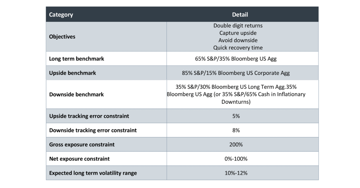
Note there is approximate symmetry of +/- 20% equity exposure around the upside and downside components of the secondary benchmark. The economic environment sets the weight between the upside and downside components. Therefore, symmetry is preserved. There is a skew in upside and downside TE as required, and over the cycle we expect this to average around 6%. Also as required this is greater than the secondary benchmark TE versus the primary benchmark, which is approximately 2%.
In this way, all of the above principles are satisfied structurally. We now go on to illustrate the benefit of this approach in delivered return.
Illustrating the benefits of the PEP Mandate Structure on Delivered Performance
In order to illustrate the benefits of this approach, we seek to show analysis that takes precisely the same views, but applies them in three different frameworks:
A traditional mandate structure with a 65/35 benchmark as above, with a static TE constraint of 6% p.a..
The same mandate structure but with a maximum TE of 10% p.a..
The PEP Portfolio Construction Framework – as described above, this involves the use of a Dynamic Benchmark, and dynamic TE constraints.
We have developed the investment views by simulating whether we are overweight or underweight in each market and forcing a probability of being right or wrong. The tables below illustrate a series of simulated results but with different levels of accuracy in decision making. In the first instance we show if decisions are made with 55% accuracy (i.e. majority right). In the second table we show if decisions are made with 45% accuracy (i.e. majority wrong).
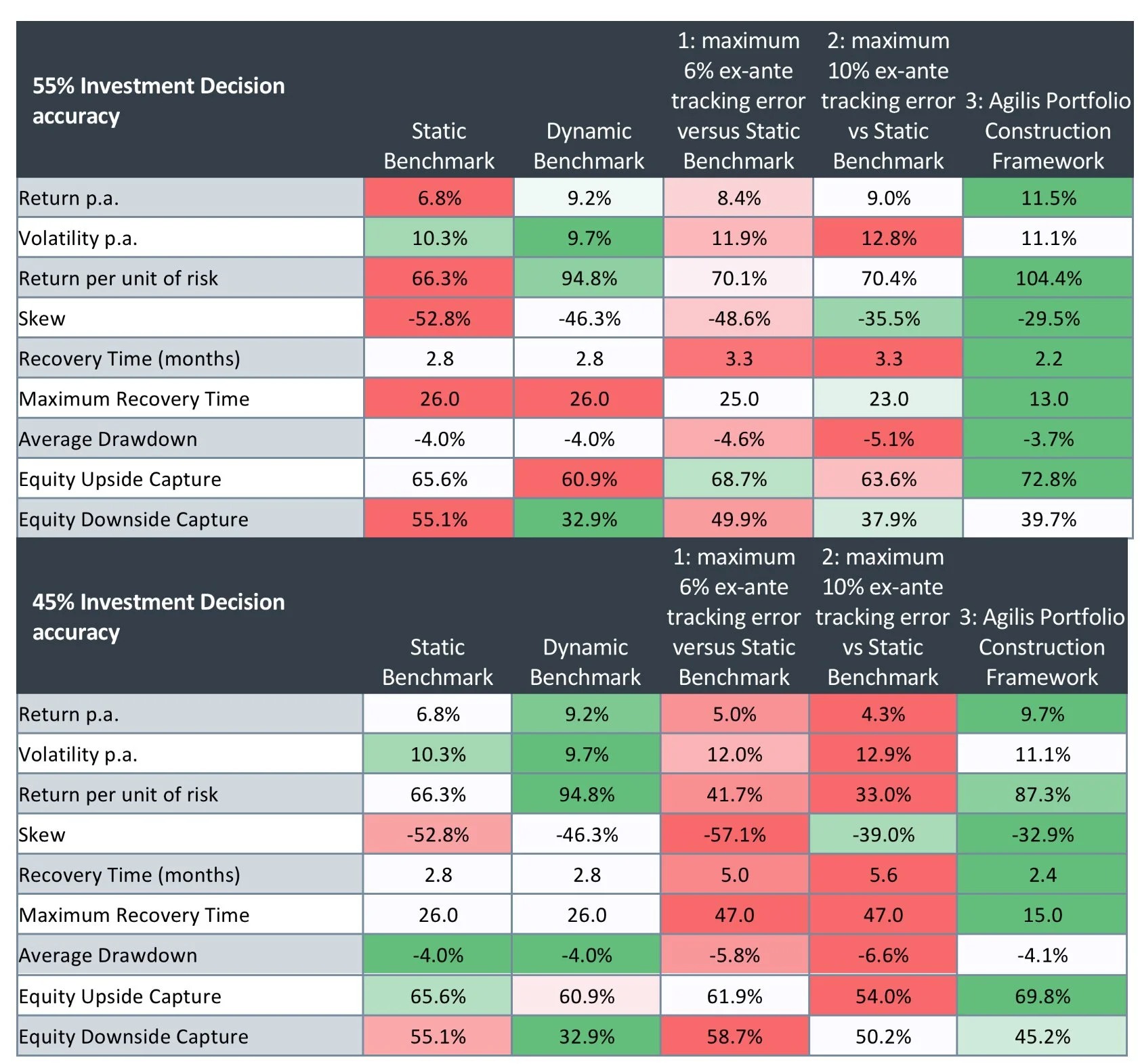
Source: Figures produced by PEP based on a simulated decision-making process from 01/01/1999 to 09/30/2023. The static benchmark is 65% S&P500, 35% Bloomberg US Long Treasury Total Return Index in USD. Dynamic Benchmark is based on PEP proprietary models. Simulated performance is no indication of future results.
As expected, the table illustrates strong characteristics for the PEP Portfolio Construction Framework across the board. Remember – each of the three portfolios are based on the exact same decisions in terms of timing, just with different portfolio construction constraints which influence position sizing. The following points are worthy of drawing out on the PEP Framework:
Returns are very strong – double digits – with a 55% chance of being right.
The efficiency of return is very strong, as is upside/downside capture.
Worst recovery time is around one year, and half that of the benchmark.
The PEP approach copes far better with weak asset manager decisions (modelled as 45% chance of being right).
The point we are trying to illustrate here is that the consistent design of the constraints is as important as the views themselves, in the process of translating them into client requirements. This is therefore the most important step in risk management – after all, risk management should be focused on mitigating the risk of not delivering on client objectives.
Summary
In this paper, we have set out the logic in the development of our Portfolio Construction Framework, tied to client objectives. The purpose of this is how to most effectively translate our views into a portfolio that has the greatest likelihood of delivering on those client objectives.
We have also illustrated with a consistent set of investment views how our Framework improves the delivery on client objectives compared to other methodologies. We believe this should give investors confidence in the portfolio construction step of our process.
Appendix – Skew impact on portfolio objectives
A factor that is often under-appreciated in its effect on portfolio results is skew.
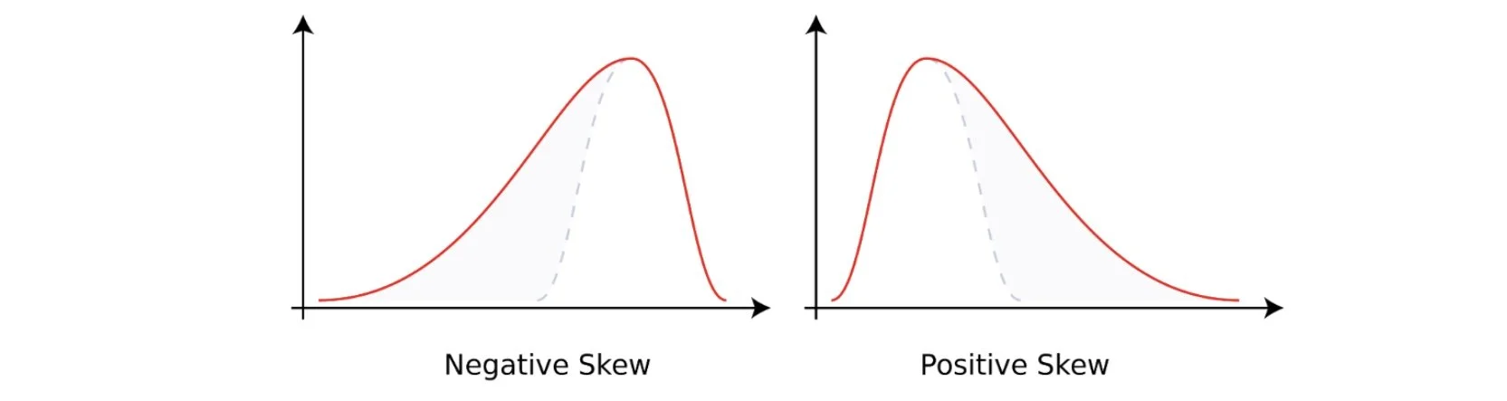
Skew is a statistical concept that describes how a return distribution “leans”. If the distribution leans to the right, then it is positively skewed, and to the left it is negatively skewed.
One of the big problems with beta is return distributions are negatively skewed. This creates a problem that cannot be solved well by running at a high Sharpe ratio (the purpose of which is different in any event, as described above). The table below illustrates this point very well for a number of theoretical strategies.
Critically, it is important to understand that most risk markets (including equities) come with negative skew. This is a bad thing for both downside risk and recovery time, as well as negatively impacting long-term returns. The analysis in the table below illustrates.
Analysis of efficiency for different Sharpe Ratios and Skew
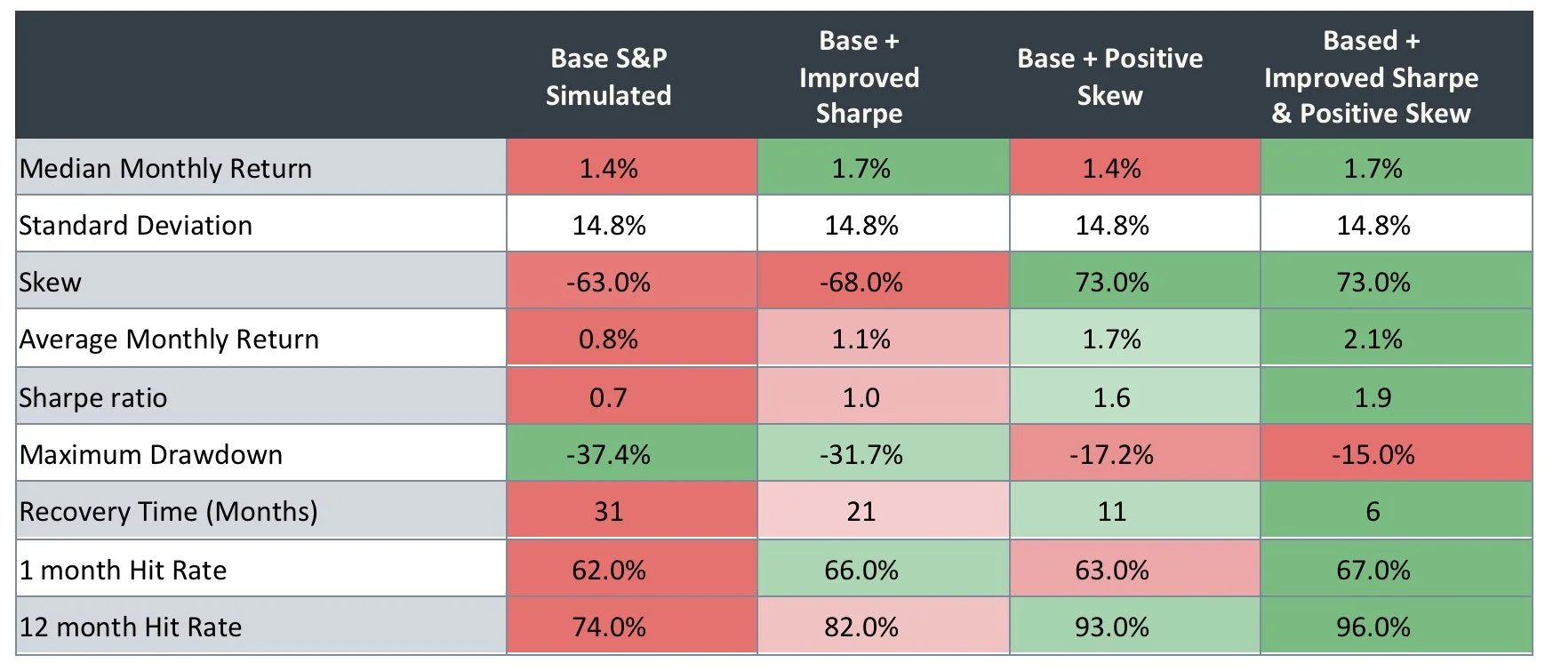
Source: Figures produced by PEP based on simulated data. Simulated performance is no indication of future results.
There is a lot of information in this table that bears explanation. Note that we have shown the median and the realized returns. The reason for this is that, for a given (fixed) median return, adding or subtracting skew has an effect on the realized return. So, where skew is strongly positive, the realized return will be greater than that implied by the median return, and vice-versa.
The first column aims to mimic the characteristics of the S&P, which is negatively skewed. We are focused in particular on the effect of Sharpe ratio and skew on the drawdown and recovery time statistics.
Columns 2 and 3 are instructive in that they look respectively at evolving Column 1 through increasing skew and then separately increasing the Sharpe ratio. Both have a positive effect on drawdown (DD) and recovery time, but the effect of skew on its own is far greater.
But following the logic from above, if we can use macro decision making to improve the Sharpe Ratio to the extent of Column 2, and somehow turn the skew positive, then recovery time is cut by 80% (compared to the S&P) and the maximum drawdown is cut by nearly two-thirds.
But how would we make skew positive? One the ways this can be done is through the dynamic secondary benchmark process described in the body of this document. It has the effect of reducing the allocation to risk assets, on average, at times when the exposure to downside is greatest. It is these downside events that create the negative skew, and as such cutting exposure to them improves the skew.
The corollary is that simply being right on average, in investment decision-making terms, does not necessarily imply that there will be positive skew. The critical thing is that great investment decisions – the “fuel” of an investment process – are used in a portfolio construction process (how “the car is engineered”) that aims to deliver positive skew. This has particularly positive effects on long-term returns and recovery time, more so than just improving the Sharpe Ratio alone.
We cover the problem with negative skew and some practical ways to address it in subsequent papers.
CONFIDENTIAL INFORMATION: The information herein has been provided solely to the addressee in connection with a presentation by Public Equity Partners LLC on condition that it not be shared, copied, circulated or otherwise disclosed to any person without the express consent of Public Equity Partners LLC.
INVESTMENT ADVISOR: Investment advisory services are provided by Public Equity Partners LLC, an investment advisor registered with the US Securities and Exchange Commission.
SIMULATED PERFORMANCE: The simulated performance was derived from the retroactive application of a model with the benefit of hindsight. Performance results do not represent actual trading. Performance does not include material economic and market factors that might have impacted the adviser's decision making when using the model to manage actual strategies. Performance does not reflect the deduction of advisory fees, brokerage or other commissions, mutual fund exchange fees, and other expenses a client may be required to pay.
PAST PERFORMANCE IS NOT AN INDICATION OF FUTURE RESULTS.
SECURITY INDICES: This presentation includes data related to the performance of various securities indices which may provide an appropriate basis for comparison with underlying investments and the client’s total investment portfolio. The performance of securities indices is not subject to fees and expenses associated with investment funds. Investments cannot be made directly in the indices. The information provided herein has been obtained from sources which Public Equity Partners LLC believes to be reasonably reliable but cannot guarantee its accuracy or completeness.
Actuarial and investment consulting - Macro investment strategies Pension annuity purchases - Pension plan termination - Derivative strategies - Pooled employer plan consulting - OCIO