
Macro Approach to Portfolio Construction & Engineering: Primary Benchmark
Primary Benchmark Design
This paper extends the thinking presented in our Portfolio Construction & Engineering paper and is therefore the second in a series of papers describing the underpinning of our investment process.
In our first paper, we presented an argument about the importance of engineering when delivering on client objectives. The result was that we argue for a mandate structure that has:
Primary and secondary benchmarks
Varying tracking error constraints relative to the secondary benchmark – specifically higher tracking error flexibility in downside environments than in upside environments
There are other influences on the specific mandate proposals, but the essence of the mandate structures is captured in these two principles.
We used a 65/35 Equity/bond benchmark as the primary benchmark used in the paper for analysis. However, this benchmark was asserted without argument. This is in part because of its prevalence in the industry, and as such it represents a useful starting point. But in this paper, we intend to relax this assumption and think about the purpose of the primary benchmark, given the assumption that this mandate structure is optimal (this is a reverse of the argument made in the previous paper). We therefore seek to examine whether the 65/35 benchmark is optimal, or if there is a more effective alternative.
There are inter-relationships between the primary benchmark and mandate design that cannot be ignored. For example, if we conclude that 50/50 is a better benchmark, we may need to re-examine what we mean by upside capture and where we set the secondary benchmark relative to the primary. But these considerations follow from the development of the primary benchmark itself. The question in front of us is how to think about the role of the primary benchmark and what role it fulfils in the context of the mandate structure we have now developed.
The structural location of the equity allocation
It is perhaps simpler to think of the benchmark as driven by where to set the equity allocation. This is the biggest determinant of the benchmark risk in most mandates. Three simple examples illustrate the point.
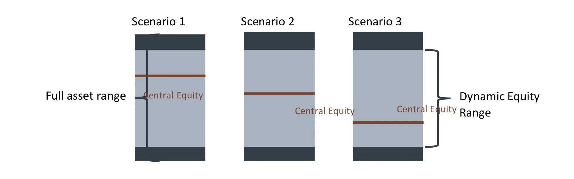
The first example is what we created in the previous paper. The second puts the equity allocation in the middle of the dynamic range and gives flexibility around this. The third puts equity allocation lower, and allows the range to skew upwards, based on dynamic decision making.
Rational arguments can be made for each of these approaches. For example, the third represents a desire to maintain a long term more defensive position but is prepared to allow the allocation to rise significantly, if the economic environment suggests this is logical.
However, this is an argument based on utility – what we are looking for is the dominant argument in the absence of these types of preferences. If all we cared about were the four objectives set out in the previous paper, what implication would that have on the location of the primary benchmark equity allocation?
As a reminder, the four objectives are:
Return – for example, produce a return of 10% per annum or more over rolling three- or five-year periods. Or, outperform the primary benchmark index by 2%-3% per annum over the same horizon.
Upside – capture the upside in market returns (primary benchmark returns) when it is available.
Downside – avoid the losses in market/benchmark returns.
Recovery time – minimize recovery time.
In the previous paper, we showed that successfully delivering on the upside and downside objectives has the implication of delivering on the other two – therefore focusing on what leads more effectively to success on these measures is key to achieving all four.
Following this logic, a more specific question is “what is the role of the primary benchmark in making it more likely that we will achieve these two objectives”?
From a pure return perspective, the heavy lifting on these two objectives (upside and downside) is done by the secondary benchmark and the quality of the investment views put into the mandate itself. Therefore, we would argue that the main purpose of the primary objective is to mitigate the risk of error in the secondary objective and/or investment views.
A simple example illustrates. If the primary benchmark equity allocation is set at 50%, there is more chance of being wrong on the upside than if the allocation is set at 65%. This is for two reasons:
The primary benchmark influences the equity allocation in the defensive environment – the higher the primary allocation, the higher the allocation in the defensive secondary benchmark.
The primary benchmark is a floor for the portfolio allocation made by dynamic decision making. So if the portfolio manager gets the view wrong, and underweights against the secondary benchmark (even if the latter is correct) then the lowest allocation that can be held is the primary benchmark allocation.
Clearly this works both ways – the higher the primary benchmark equity allocation is set, the better the risk position for the upside environment but the worse it is in the downside. Therefore, the question is how most effectively to trade these off. That is the central question that faces us in primary benchmark design. If we get our decision making wrong, would we prefer on average to err on the side of being longer equities, more balanced or lower risk?
The table below shows some performance statistics for the US equity market, the global equity market and an aggregate index of US bonds since 1993.
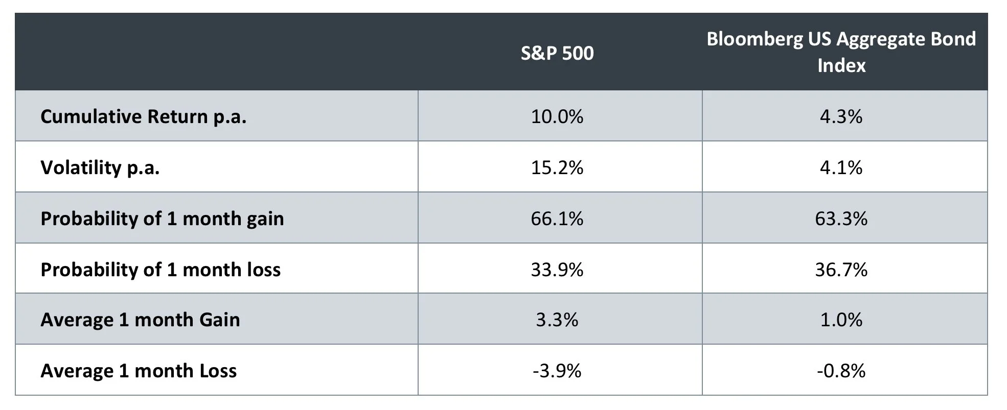
Source: Source: Bloomberg from November 1993 to November 2023. All figures shown in USD. Past performance is no indication of future results.
These statistics are helpful because they allow us to perform some simple analysis, where we assume we are holding a mix of equities and bonds. This analysis seeks to set the allocation to equities in order to equate to the “value” of the economic loss from both upside (return relative to equities) and downside (return relative to cash). To account for the diversification effect between equities and bonds, we calculate the performance of the benchmark for different allocations to equities. We then calculate the average loss relative to both 100% equities and zero (to capture the effect of absolute losses). Mathematically this is a version of Minmax – we minimize the maximum loss contribution.
The chart below shows the corresponding numbers for different benchmark weightings to equities and bonds.
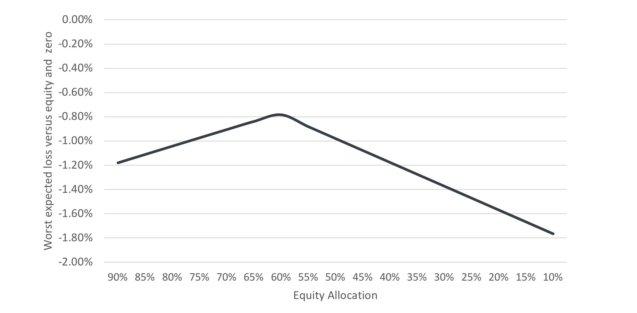
Source: Bloomberg using data from November 1993 to November 2023. All returns calculated in USD. Past and simulated performance is no indication of future results.
It is important in these situations not to be unduly precise as no model is perfect and in particular, these figures can vary depending on the time horizon being analyzed. In almost all cases though, this zone of optimality sits between 55% and 70% equity.
Implications of the analysis
The zone of optimality does give us a clear signal that, of the three types approaches we identified earlier, there is a logic for being overweighted to equities within the primary benchmark. The question now is whether we can be more specific within the range based on other influences.
The key consideration, because of the overweighting towards equities, is the potential risk to the downside that this creates. As we established earlier, the greater risk from overweighting equities within the primary benchmark is achieving success in downside environments. However, there is another more complex issue that it is worth considering and that is the potential for undue reliance on investment views on one side or the other (upside or downside).
It is perhaps obvious that, if we set the primary benchmark allocation to equities at 100%, we are completely exposed to the quality of our views on the downside, and our upside views are irrelevant. The converse is clearly true if we set the equity allocation at 0%. The effect of this is to introduce skew into the quality of the added value generated from all of our views.
We are able to quantify the effect on this by considering the “volatility” of the alpha generated through investment decisions (for simplicity we are assuming that both the secondary benchmark and active decisions relative to that are aggregated). The chart below shows the resulting volatility of alpha for different equity allocations, based on the realized probability of loss for these portfolios since 1993 (as with the above analysis, other periods show a comparable result).
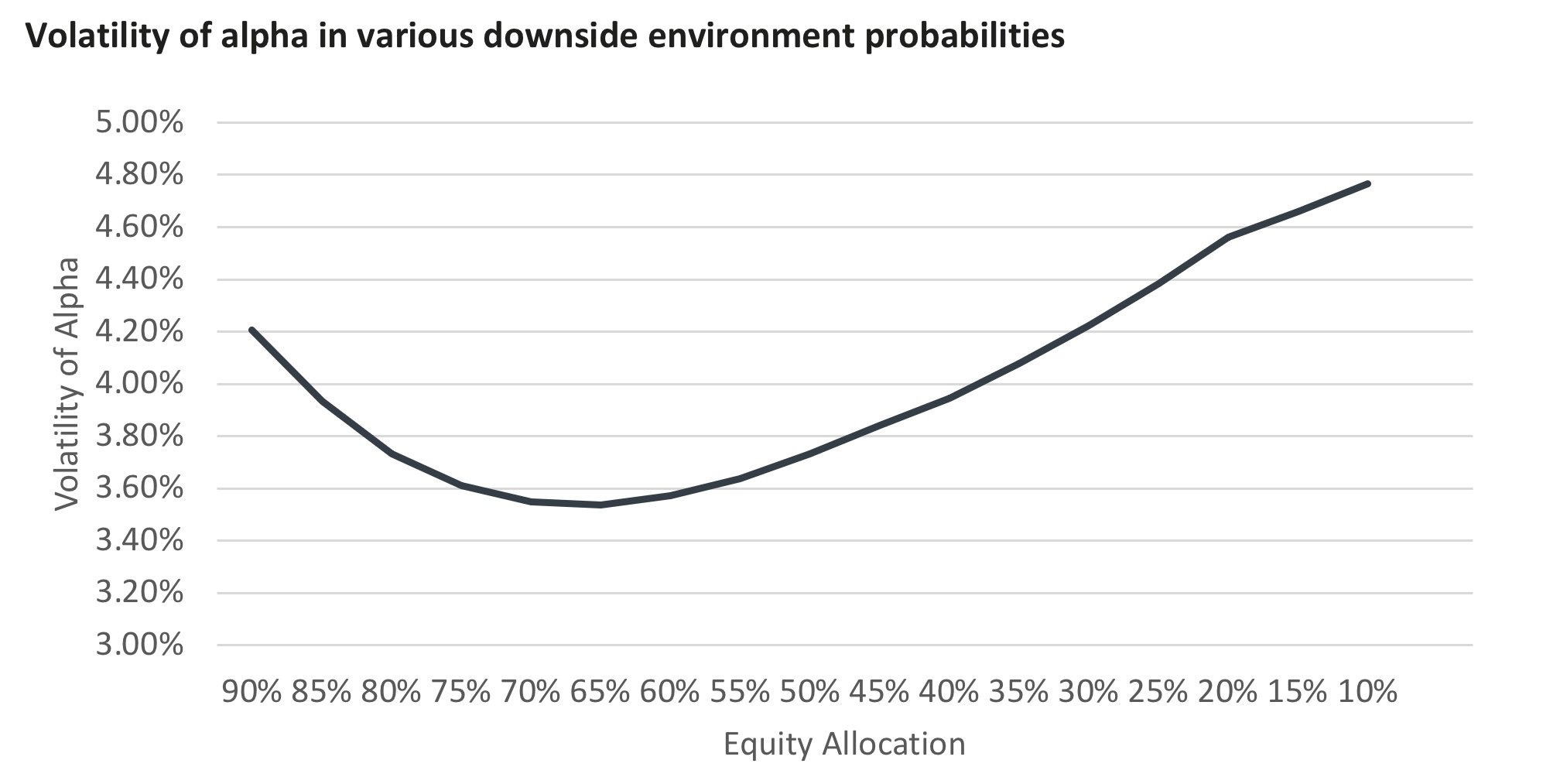
Source: Bloomberg using data from November 1993 to November 2023 based on the S&P500. All returns calculated in USD. Past and simulated performance is no indication of future results.
What is clear from the analysis is that there is again a zone of optimality, this time between 65% and 70%. In this instance, we would tend to argue that lower is slightly better, as it introduces robustness if our beta assumption is less reliable. Nonetheless, any of the allocations in this range appear to do a good job of keeping the alpha quality balanced in downside environments.
The analysis presented in the previous section concluded that a zone of optimality would be in the range of 55-70% equity allocation. Combining this with the analysis in this section, we can narrow this to 65%-70%. Nonetheless, based on the comment about a slightly lower allocation managing the risk of our beta assumptions (probability of loss) being optimistic, we would argue that 65% is broadly optimal. The other reason for being lower in the range relates to the development of the mandate structure itself. A higher equity allocation will result in a greater contribution to tracking error on the downside from the secondary benchmark, which in turn will require even more tracking error flexibility to be given the manager relative to this. Therefore, there is a marginal loss of control for the investor from higher equity allocations. This is minor but within a zone of optimality will argue for a lower allocation to equities.
Conclusion
The analysis presented in this paper has focused on determining whether there is an analytical basis for an optimal primary benchmark position. Our analysis focused on:
Applying a minimax approach to the probability of loss versus equities and cash
Understanding the quality of alpha that results from the selection of a primary benchmark equity allocation
Based on this, we conclude a 65%/35% primary benchmark is broadly optimal.
This result is especially interesting because we have not needed to deploy any preferences in its development. We are arguing that, based on balancing the various analytical influences on mandate and benchmark structure, if the objective is to produce consistent and significant long term returns our proposed mandate structure is optimal. Specifically, this involves:
a 65/35 primary benchmark
a secondary benchmark that allows the equity allocation to vary relative to the primary benchmark
tracking error constraints relative to this secondary benchmark that are skewed – lower on the upside and more flexible on the downside
This mandate structure forms the basis of our Multi Asset Growth Strategy.
CONFIDENTIAL INFORMATION: The information herein has been provided solely to the addressee in connection with a presentation by Public Equity Partners LLC, on condition that it not be shared, copied, circulated or otherwise disclosed to any person without the express consent of Public Equity Partners LLC.
INVESTMENT ADVISOR: Investment advisory services are provided by Public Equity Partners LLC, an investment advisor registered with the US Securities and Exchange Commission.
SIMULATED PERFORMANCE: The simulated performance was derived from the retroactive application of a model with the benefit of hindsight. Performance results do not represent actual trading. Performance does not include material economic and market factors that might have impacted the adviser's decision making when using the model to manage actual strategies. Performance does not reflect the deduction of advisory fees, brokerage or other commissions, mutual fund exchange fees, and other expenses a client may be required to pay.
PAST PERFORMANCE IS NOT AN INDICATION OF FUTURE RESULTS.
SECURITY INDICES: This presentation includes data related to the performance of various securities indices which may provide an appropriate basis for comparison with underlying investments and the client’s total investment portfolio. The performance of securities indices is not subject to fees and expenses associated with investment funds. Investments cannot be made directly in the indices. The information provided herein has been obtained from sources which Public Equity Partners LLC. believes to be reasonably reliable but cannot guarantee its accuracy or completeness.
Actuarial and investment consulting - Macro investment strategies Pension annuity purchases - Pension plan termination - Derivative strategies - Pooled employer plan consulting - OCIO